Soft clustering

Like HDBSCAN*, PLSCAN can compute soft membership probabilities for each point.

import numpy as np
import matplotlib.pyplot as plt
from fast_plscan import PLSCAN

plt.rcParams["figure.dpi"] = 150
plt.rcParams["figure.figsize"] = (2.75, 0.618 * 2.75)

data = np.load("data/clusterable/sources/clusterable_data.npy")

Import the all_points_membership_vectors function from the prediction module to compute membership probabilities. The implementation follows the same ideas as HDBSCAN* soft clustering, except that it uses mutual reachability distances rather than raw pairwise distances. See the HDBSCAN* documentation for additional details.

from fast_plscan.prediction import all_points_membership_vectors

c = PLSCAN(min_samples=2, min_cluster_size=10).fit(data)
memberships = all_points_membership_vectors(c)

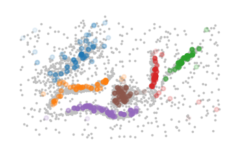
Some points are always treated as noise in this implementation. These points have zero membership values in all columns because they are direct descendants of the phantom root. We cannot reliably recover where they should attach in the hierarchy, so they remain noise.

plt.figure()
noise = np.all(memberships == 0, axis=1)
cs = memberships[~noise].argmax(axis=1)
probs = memberships[~noise, cs]
plt.scatter(*data[noise, :].T, s=0.5, color="silver")
plt.scatter(*data[~noise, :].T, s=1, c=cs, alpha=probs, vmax=9, cmap="tab10")
plt.axis("off")
plt.show()

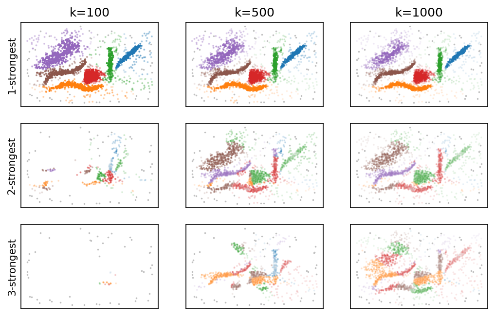
Precomputed distance inputs

Unlike the HDBSCAN* implementation, we also support computing membership vectors for precomputed sparse distance matrices. The more neighbors are present, the more membership information can be extracted. This is visible in the visualization below as more information in the second and third strongest memberships.

from pynndescent import NNDescent


plt.figure(figsize=(2.75 * 3, 0.618 * 2.75))
plt.gcf().set_size_inches(2.75 * 3, 0.618 * 2.75 * 3)

for i, k in enumerate([100, 500, 1000], 1):
    nn = NNDescent(data, metric="euclidean", n_neighbors=k)
    neighbors, distances = nn.neighbor_graph

    c = PLSCAN(metric="precomputed").fit((distances, neighbors))
    sparse_memberships = all_points_membership_vectors(c)

    noise = np.all(sparse_memberships == 0, axis=1)
    sorted_labels = np.argsort(sparse_memberships, axis=1)[:, ::-1]
    n = sparse_memberships.shape[0]

    for rank in range(3):
        labels = sorted_labels[:, rank]
        alpha = sparse_memberships[np.arange(n), labels]

        plt.subplot(3, 3, rank * 3 + i)
        plt.scatter(*data[noise, :].T, s=0.5, color="silver")
        plt.scatter(
            *data[~noise, :].T,
            s=1,
            c=labels[~noise],
            alpha=alpha[~noise],
            vmax=9,
            cmap="tab10",
        )
        if rank == 0:
            plt.title(f"k={k}")
        if i == 1:
            plt.ylabel(f"{rank + 1}-strongest")
        plt.xticks([])
        plt.yticks([])
plt.show()

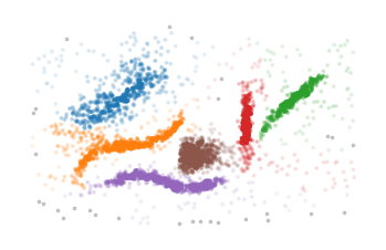
Memberships of unseen points

The membership_vectors function extends soft clustering to unseen feature vectors. Each new point is attached to the fitted structure through its nearest mutual-reachability neighbor in the training set, then both distance-to-exemplar and topology-based weights are combined in the same way as for training points. The output has the same semantics as all_points_membership_vectors: each row sums to at most the point’s probability of belonging to any selected cluster.

from fast_plscan.prediction import membership_vectors

c = PLSCAN(min_samples=2, min_cluster_size=10).fit(data)

# Use a held-out slice as unseen points
rng = np.random.Generator(np.random.PCG64(25))
X_new = rng.choice(data, size=200, replace=False) + 0.015
mv = membership_vectors(c, X_new)


plt.figure()
noise = np.all(mv == 0, axis=1)
cs = mv[~noise].argmax(axis=1)
probs = mv[~noise, cs]
plt.scatter(*data.T, s=0.5, color="silver", zorder=0)
plt.scatter(*X_new[~noise].T, s=8, c=cs, alpha=probs, vmax=9, cmap="tab10", zorder=1)
plt.axis("off")
plt.show()