Parameter sensitivity analysis
The cluster selection strategies notebook demonstrates PLSCAN is less sensitive to the min_samples parameter (\(k\)) than HDBSCAN*. This notebook runs a more comprehensive parameter sensitivity analysis to determine whether that pattern holds on other datasets. This parameter sensitivity analysis tells us how the clustering quality changes as a result of changing \(k\). The resulting value is independent of \(k\) itself. Instead they
relate to a change in \(k\): \(\Delta k\)!
We apply the analysis Peng et al. 2022 used to evaluate their clustering algorithm. They modified a “Latin-Hypercube One-factor-At-a-Time (LH-OAT)” analysis. This sounds more complicated than it is, especially for algorithms with a single parameter. The steps are as follows:
Choose a parameter \(k\) and divided its value-space in regularly sized segments.
Choose a constant perturbation \(\Delta v\) to evaluate.
Sample values \(v\) in each segment. We denote the set of sampled values with \(V\).
Perturb the sampled values with \(\pm \Delta v\), randomly choosing the positive or negative direction.
Compute the algorithm’s clustering quality scores at \(v\) and \(v \pm \Delta v\). For example, using the ARI. We denote this score as \(ARI(k=v)\), indicating a score at parameter value \(k=v\).
Compute the sensitivity at \(\Delta v\) using:
\[s_{\Delta v} = \frac{1}{|V|} \sum_{v \in V} \left|\frac{ARI(k=v \pm \Delta v) - ARI(k=v)} {ARI(k=v \pm\Delta v) + ARI(k=v)}\right|.\]
We want to evaluate the sensitivity for multiple perturbation sizes \(\Delta v\), algorithm configurations, and datasets. Our implementation splits the work in three stages and considers several clustering quality measures:
Sample the parameter and perturbations, collecting all parameter values to evaluate.
Compute the algorithms’ clustering quality measures values on all datasets with the collected parameter values. Store these values!
Use the computed quality measures values to compute average sensitivities for each perturbation size.
[1]:
import warnings

import os
import time
import numpy as np
import pandas as pd
from tqdm import tqdm
from itertools import product
from scipy.stats import rankdata
from collections import defaultdict
from sklearn.datasets import fetch_openml, load_iris as sk_load_iris

from umap import UMAP
from lensed_umap import embed_graph

from hdbscan import HDBSCAN
from fast_plscan import PLSCAN
from sklearn.metrics import adjusted_rand_score, homogeneity_score, completeness_score

from lib.plotting import sns, plt, mpl, lighten, frame_off
from lib.drawing import regplot_lowess_ci


plt.rcParams["figure.dpi"] = 150
plt.rcParams["figure.figsize"] = (2.75, 0.618 * 2.75)
1. Sample parameter values and perturbations
This cell performs the parameter value sampling and applies perturbations at multiple sizes. The process is repeated five times (vectorized) and all unique parameter values required for the sensitivity computation are collected.
Perturbations that create invalid values (<2) are ignored!
[2]:
# configuration
repeats = 5
num_segments = 10
min_sample_range = (2, 50)
deltas = np.array([[2], [5], [10]])

# sampled values
segments = np.linspace(*min_sample_range, num_segments + 1, dtype=int)
samples = np.random.uniform(segments[:-1], segments[1:], size=(repeats, num_segments))
min_sample_sizes = np.round(samples).astype(int).T

# perturbed values
directions = np.random.choice((-1, 1), size=(deltas.shape[0], num_segments, repeats))
perturbations = directions * deltas[:, :, np.newaxis]
new_values = min_sample_sizes[np.newaxis, :, :] + perturbations

# all values to evaluate
all_values = np.concatenate((min_sample_sizes.flatten(), new_values.flatten()))
all_values = np.unique(all_values)
all_values = all_values[(all_values >= 2)]

np.save("data/generated/benchmark_sensitivity_deltas.npy", deltas)
np.save("data/generated/benchmark_sensitivity_min_sizes.npy", min_sample_sizes)
np.save("data/generated/benchmark_sensitivity_perturbed_values.npy", new_values)
2. Compute quality measures
This stage computes clustering quality measures at the sampled parameter values.
First, we configure the datasets. This step assumes all dataset have been downloaded and pre-processed before running this notebook. See instructions at docs/data/[data-set]/README.md!
[3]:
def load_iris():
    X, y = sk_load_iris(return_X_y=True)
    return X, y.astype(np.intp)


def load_mnist():
    X, y = fetch_openml("mnist_784", version=1, return_X_y=True)
    return X, y.cat.codes.to_numpy().astype(np.intp)


def load_fashion_mnist():
    X, y = fetch_openml("Fashion-MNIST", version=1, return_X_y=True)
    return X, y.cat.codes.to_numpy().astype(np.intp)


def local_data_loader(folder):
    """Load data from a specified folder in the data directory.

    See `data/[data-set]/README.md` for processing details.
    """
    X_path = f"data/{folder}/generated/X.npy"
    y_path = f"data/{folder}/generated/y.npy"
    if not (os.path.exists(X_path) or os.path.exists(y_path)):
        raise FileNotFoundError(f"Data not found in folder: {folder}")

    def load_data():
        X = np.load(X_path)
        y = np.load(y_path)
        return X, y.astype(np.intp)

    return load_data


data_configs = dict(
    iris=load_iris,
    mnist=load_mnist,
    fashion_mnist=load_fashion_mnist,
)

for folder in os.listdir("data"):
    if folder in ["generated", "clusterable"]:
        continue
    if not os.path.isdir(os.path.join("data", folder)):
        continue

    try:
        loader = local_data_loader(folder)
        data_configs[folder] = loader
    except FileNotFoundError:
        warnings.warn(
            f"Skipping {folder}. See "
            f"`data/{folder}/README.md` for download instructions."
        )
Next, we implement the clustering quality measures:
[4]:
def compute_quality(true_labels, predicted_labels):
    non_noise = predicted_labels != -1

    ari = adjusted_rand_score(true_labels[non_noise], predicted_labels[non_noise])
    homogeneity = homogeneity_score(true_labels[non_noise], predicted_labels[non_noise])
    completeness = completeness_score(
        true_labels[non_noise], predicted_labels[non_noise]
    )
    mutual_info = 2.0 * homogeneity * completeness / (homogeneity + completeness)
    noise_fraction = 1 - non_noise.sum() / len(predicted_labels)
    return ari, homogeneity, completeness, mutual_info, noise_fraction
Then, we create functions that evaluate the algorithms. These functions return one or more records identifying the dataset, algorithm configuration, and resulting quality scores. For PLSCAN, we compute scores for its top-\(n\) layers:
[5]:
def evaluate_hdbscan(X, y, data_name, k, alg_name, params, post_params):
    with warnings.catch_warnings():
        warnings.simplefilter("ignore")
        start = time.perf_counter()
        labels = HDBSCAN(min_samples=k, min_cluster_size=k, **params).fit_predict(X)
        duration = time.perf_counter() - start
    ari, homogeneity, completeness, mutual_info, noise_fraction = compute_quality(
        y, labels
    )
    return [
        dict(
            ari=ari,
            homogeneity=homogeneity,
            completeness=completeness,
            mutual_info=mutual_info,
            noise_fraction=noise_fraction,
            data_set=data_name,
            compute_time=duration,
            k=k,
            alg_id="_".join([alg_name] + [f"{v}" for v in params.values()]),
            alg_config={"algorithm": alg_name, **params},
        )
    ]
[6]:
def evaluate_plscan(X, y, data_name, k, alg_name, params, post_params):
    # Compute PLSCAN layers
    start = time.perf_counter()
    c = PLSCAN(min_samples=k, min_cluster_size=k, **params).fit(X)
    duration = time.perf_counter() - start
    layers = c.cluster_layers(**post_params) or [(k, c.labels_, c.probabilities_)]

    # Rank layers by their persistence score
    sizes, pers = c._persistence_trace
    sizes = sizes if sizes.shape[0] > 0 else np.array([k], dtype=np.float32)
    pers = pers if pers.shape[0] > 0 else np.array([0.0], dtype=np.float32)
    s = [s for s, _, _ in layers]
    ranks = rankdata(-pers[np.searchsorted(sizes, s)], method="ordinal")
    records = []

    # Create a record and compute quality for each layer
    for peak, (size, labels, _) in zip(ranks, layers):
        ari, homogeneity, completeness, mutual_info, noise_fraction = compute_quality(
            y, labels
        )
        records.append(
            dict(
                ari=ari,
                homogeneity=homogeneity,
                completeness=completeness,
                mutual_info=mutual_info,
                noise_fraction=noise_fraction,
                compute_time=duration,
                data_set=data_name,
                k=k,
                alg_id="_".join(
                    [alg_name] + [f"{v}" for v in params.values()] + [f"{peak}"]
                ),
                alg_config={
                    "algorithm": alg_name,
                    **params,
                    "peak": peak,
                    "birth_size": size,
                },
            )
        )
    return records
Next, we specify the algorithm–parameter configurations. We want to evaluate all parameter-value combinations. In this case, only the cluster selection strategies vary.
[7]:
# Configurations
algorithms = dict(plscan=evaluate_plscan, hdbscan=evaluate_hdbscan)
in_params = defaultdict(
    dict,
    plscan=dict(
        persistence_measure=[
            "size",
            "distance",
            "density",
            "size-distance",
            "size-density",
        ]
    ),
    hdbscan=dict(cluster_selection_method=["leaf", "eom"]),
)
post_params = defaultdict(dict, plscan=dict(max_peaks=[5]))
algorithm_configs = [
    (
        fun,
        name,
        {param: value for param, value in zip(in_params[name].keys(), param_values)},
        {
            param: value
            for param, value in zip(post_params[name].keys(), post_param_values)
        },
    )
    for name, fun in algorithms.items()
    for param_values in product(*in_params[name].values())
    for post_param_values in product(*post_params[name].values())
]
Finally, run all algorithm–dataset–\(k\) combinations (takes about 3 hours).
We project all datasets down to 50 dimension using UMAP. We slowly increase UMAP’s repulsion strength parameter to avoid self-intersections in the layout. The set_op_mix_ratio parameter increases cluster separation in the layout. This step could be tuned for each dataset to increase performance. We are mostly interested in parameter stability, though, so these settings are good enough.
[8]:
records = []

pbar = tqdm(total=len(data_configs) * len(all_values) * len(algorithm_configs))
for data_name, loader in data_configs.items():
    # Load the data
    X, y = loader()

    # Project down to 50 dimensions with UMAP.
    # Repeats the layout procedure with increasing repulsion to avoid overlaps
    with warnings.catch_warnings():
        warnings.simplefilter("ignore")
        p = UMAP(
            n_components=min(50, X.shape[1]),
            n_neighbors=min(250, X.shape[0] - 1),
            metric="cosine",
            set_op_mix_ratio=0.1,
            transform_mode="graph",
        ).fit(X)
        p = embed_graph(p, repulsion_strengths=[0.001, 0.01, 0.1, 1])
    np.save(
        f"data/generated/benchmark_sensitivity_{data_name}_embedding.npy", p.embedding_
    )

    # Evaluate the algorithms
    for k, (evaluator, alg_name, params, post_params) in product(
        all_values, algorithm_configs
    ):
        if k < X.shape[0] - 1:
            records.extend(
                evaluator(p.embedding_, y, data_name, k, alg_name, params, post_params)
            )
        pbar.update()


df = pd.DataFrame.from_records(records)
df.to_parquet("data/generated/benchmark_sensitivity.parquet")
df.head()
100%|██████████| 6307/6307 [38:22<00:00, 261.05it/s]
[8]:
| ari | homogeneity | completeness | mutual_info | noise_fraction | compute_time | data_set | k | alg_id | alg_config | |
|---|---|---|---|---|---|---|---|---|---|---|
| 0 | 0.269821 | 0.940310 | 0.401353 | 0.562580 | 0.046667 | 0.000891 | iris | 2 | plscan_size_3 | {'algorithm': 'plscan', 'persistence_measure':... |
| 1 | 0.332761 | 0.896505 | 0.434125 | 0.584979 | 0.006667 | 0.000891 | iris | 2 | plscan_size_2 | {'algorithm': 'plscan', 'persistence_measure':... |
| 2 | 0.883428 | 0.867358 | 0.865420 | 0.866388 | 0.053333 | 0.000891 | iris | 2 | plscan_size_1 | {'algorithm': 'plscan', 'persistence_measure':... |
| 3 | 0.127932 | 0.964315 | 0.326040 | 0.487315 | 0.153333 | 0.000742 | iris | 2 | plscan_distance_2 | {'algorithm': 'plscan', 'persistence_measure':... |
| 4 | 0.332761 | 0.896505 | 0.434125 | 0.584979 | 0.006667 | 0.000742 | iris | 2 | plscan_distance_3 | {'algorithm': 'plscan', 'persistence_measure':... |
2.5 Plot the results
This section plots the \(k\)–quality curves for all evaluated algorithms configurations and datasets.
First, we load the data generated by the previous steps.
[9]:
df = pd.read_parquet("data/generated/benchmark_sensitivity.parquet")
deltas = np.load("data/generated/benchmark_sensitivity_deltas.npy")
min_sample_sizes = np.load("data/generated/benchmark_sensitivity_min_sizes.npy")
new_values = np.load("data/generated/benchmark_sensitivity_perturbed_values.npy")
Then, we configure display names for the variables and values.
[10]:
def to_display_name(input):
    parts = input.split("_")
    name = parts[0].upper()
    if name == "HDBSCAN":
        name = "HDBSCAN*"
        return f"{name} ({' '.join(parts[1:])})"
    if name == "PLSCAN":
        params = [
            p.replace("-", "–").replace("density", "λ").replace("distance", "d")
            for p in parts[1:]
        ]
        return f"{name} ({' '.join(params)})"
    return input


def dataset_name(input):
    names = dict(
        iris="Iris",
        mnist="MNIST",
        fashion_mnist="Fashion-MNIST",
        articles_1442_5="Articles-1442-5",
        articles_1442_80="Articles-1442-80",
        audioset="AudioSet (music)",
        authorship="Authorship",
        cardiotocography="CTG",
        cell_cycle_237="CellCycle-237",
        cifar_10="CIFAR-10",
        ecoli="E. coli",
        elegans="C. elegans",
        mfeat_factors="Mfeat-Factors",
        mfeat_karhunen="Mfeat-Karhunen",
        newsgroups="20 Newsgroups",
        semeion="Semeion Digits",
        yeast_galactose="YeastGalactose",
    )
    return names.get(input, input)
Next, we summarize PLSCAN’s layers into the default (most-persistent) layer, and the optimal layer at each \(k\). The latter strategy mimics a workflow that manually inspects and selects a cluster layer when tuning the algorithm.
[11]:
# Create new data frame without the rows for non-default plscan layers
def digit_higher_than_one(char):
    return char.isdigit() and int(char) > 1


mask = df.alg_id.apply(lambda x: not digit_higher_than_one(x.split("_")[-1]))
df_default = df[mask].copy()
df_default.alg_id = df_default.alg_id.apply(
    lambda x: x if "plscan" not in x else "_".join(x.split("_")[:-1])
)
[12]:
# Select rows with the best plscan layer at each dataset--k
plscan_df = df.query("alg_id.str.startswith('plscan')", engine="python").copy()
plscan_df["persistence"] = plscan_df.alg_id.apply(lambda x: x.split("_")[1])
plscan_df["layer"] = plscan_df.alg_id.apply(lambda x: x.split("_")[-1])
best_layer = (
    plscan_df.groupby(["data_set", "persistence", "k"])
    .apply(lambda g: g.loc[g.ari.idxmax()], include_groups=False)
    .reset_index()
)
best_layer.alg_id = best_layer.alg_id.apply(
    lambda x: "_".join(x.split("_")[:-1] + ["top"])
)
best_layer = best_layer.drop(columns=["layer", "persistence"])
Maximum observed mutual information per dataset and algorithm:
[13]:
# Combine these dataframes
df_top = pd.concat((df_default, best_layer), ignore_index=True)
df_top.groupby(["data_set", "alg_id"]).apply(
    lambda g: g.loc[g.mutual_info.idxmax(), ["mutual_info"]],
    include_groups=False,
).reset_index().round(3).pivot(
    index="alg_id", columns="data_set", values=["mutual_info"]
)
[13]:
| mutual_info | |||||||||||||||||
|---|---|---|---|---|---|---|---|---|---|---|---|---|---|---|---|---|---|
| data_set | articles_1442_5 | articles_1442_80 | audioset | authorship | cardiotocography | cell_cycle_237 | cifar_10 | ecoli | elegans | fashion_mnist | iris | mfeat_factors | mfeat_karhunen | mnist | newsgroups | semeion | yeast_galactose |
| alg_id | |||||||||||||||||
| hdbscan_eom | 0.987 | 1.0 | 0.498 | 0.970 | 0.983 | 0.546 | 0.883 | 0.561 | 0.768 | 0.648 | 1.0 | 0.828 | 0.867 | 0.913 | 0.725 | 0.657 | 0.882 |
| hdbscan_leaf | 0.987 | 1.0 | 0.525 | 0.842 | 0.920 | 0.565 | 0.733 | 0.793 | 0.813 | 0.558 | 1.0 | 0.901 | 0.923 | 0.702 | 0.779 | 0.846 | 0.850 |
| plscan_density | 0.987 | 1.0 | 0.542 | 0.970 | 0.936 | 0.553 | 0.735 | 0.683 | 0.818 | 0.575 | 1.0 | 0.861 | 0.901 | 0.835 | 0.784 | 0.824 | 0.834 |
| plscan_density_top | 0.987 | 1.0 | 0.545 | 0.970 | 0.997 | 0.558 | 0.907 | 0.700 | 0.818 | 0.644 | 1.0 | 0.892 | 0.932 | 0.948 | 0.785 | 0.838 | 0.834 |
| plscan_distance | 0.987 | 1.0 | 0.542 | 0.970 | 0.920 | 0.303 | 0.735 | 0.410 | 0.818 | 0.552 | 1.0 | 0.723 | 0.875 | 0.835 | 0.784 | 0.737 | 0.834 |
| plscan_distance_top | 0.987 | 1.0 | 0.545 | 0.970 | 0.997 | 0.558 | 0.907 | 0.709 | 0.818 | 0.586 | 1.0 | 0.875 | 0.927 | 0.949 | 0.785 | 0.838 | 0.834 |
| plscan_size | 0.987 | 1.0 | 0.495 | 0.970 | 0.922 | 0.557 | 0.907 | 0.683 | 0.766 | 0.696 | 1.0 | 0.910 | 0.934 | 0.949 | 0.765 | 0.839 | 0.731 |
| plscan_size-density | 0.987 | 1.0 | 0.495 | 0.970 | 0.922 | 0.546 | 0.415 | 0.683 | 0.717 | 0.414 | 1.0 | 0.800 | 0.899 | 0.436 | 0.557 | 0.708 | 0.731 |
| plscan_size-density_top | 0.987 | 1.0 | 0.543 | 0.970 | 0.971 | 0.558 | 0.907 | 0.683 | 0.818 | 0.717 | 1.0 | 0.910 | 0.932 | 0.949 | 0.776 | 0.839 | 0.731 |
| plscan_size-distance | 0.987 | 1.0 | 0.495 | 0.970 | 0.922 | 0.303 | 0.415 | 0.410 | 0.717 | 0.414 | 1.0 | 0.658 | 0.875 | 0.436 | 0.583 | 0.708 | 0.731 |
| plscan_size-distance_top | 0.987 | 1.0 | 0.543 | 0.970 | 0.971 | 0.558 | 0.907 | 0.709 | 0.818 | 0.717 | 1.0 | 0.864 | 0.921 | 0.949 | 0.776 | 0.839 | 0.775 |
| plscan_size_top | 0.987 | 1.0 | 0.538 | 0.970 | 0.971 | 0.558 | 0.907 | 0.683 | 0.814 | 0.717 | 1.0 | 0.910 | 0.934 | 0.949 | 0.783 | 0.839 | 0.731 |
ARI values at \(k=4\) for the default layers:
[14]:
tab = (
    df_top.query("k==4")
    .pivot(index="data_set", columns="alg_id", values=["ari"])
    .round(2)
)
columns = [
    "hdbscan_eom",
    "hdbscan_leaf",
    "plscan_size",
    "plscan_size-distance",
    "plscan_size-density",
    "plscan_distance",
    "plscan_density",
]
tab[[("ari", c) for c in columns]]
[14]:
| ari | |||||||
|---|---|---|---|---|---|---|---|
| alg_id | hdbscan_eom | hdbscan_leaf | plscan_size | plscan_size-distance | plscan_size-density | plscan_distance | plscan_density |
| data_set | |||||||
| articles_1442_5 | 0.96 | 0.56 | 0.84 | 0.99 | 0.99 | 0.99 | 0.99 |
| articles_1442_80 | 0.96 | 0.42 | 0.92 | 0.99 | 0.99 | 0.99 | 0.99 |
| audioset | -0.00 | 0.02 | 0.09 | 0.14 | 0.14 | 0.03 | 0.03 |
| authorship | 0.98 | 0.15 | 0.88 | 0.98 | 0.98 | 0.98 | 0.98 |
| cardiotocography | 0.15 | 0.07 | 0.37 | 0.68 | 0.86 | 0.59 | 0.08 |
| cell_cycle_237 | 0.50 | 0.19 | 0.50 | 0.20 | 0.50 | 0.20 | 0.50 |
| cifar_10 | 0.59 | 0.01 | 0.89 | 0.17 | 0.17 | 0.02 | 0.02 |
| ecoli | 0.35 | 0.26 | 0.48 | 0.35 | 0.65 | 0.35 | 0.25 |
| elegans | 0.55 | 0.09 | 0.52 | 0.38 | 0.38 | 0.65 | 0.65 |
| fashion_mnist | 0.34 | 0.01 | 0.52 | 0.15 | 0.15 | 0.01 | 0.01 |
| iris | 0.57 | 0.29 | 0.88 | 0.57 | 0.88 | 0.57 | 0.30 |
| mfeat_factors | 0.71 | 0.15 | 0.85 | 0.41 | 0.41 | 0.41 | 0.15 |
| mfeat_karhunen | 0.69 | 0.15 | 0.91 | 0.63 | 0.63 | 0.63 | 0.17 |
| mnist | 0.66 | 0.01 | 0.96 | 0.21 | 0.21 | 0.01 | 0.01 |
| newsgroups | 0.16 | 0.06 | 0.25 | 0.25 | 0.09 | 0.07 | 0.07 |
| semeion | 0.15 | 0.19 | 0.70 | 0.32 | 0.32 | 0.32 | 0.20 |
| yeast_galactose | 0.90 | 0.27 | 0.75 | 0.75 | 0.75 | 0.75 | 0.28 |
Compute times for the datasets (only default PLSCAN computation, not the layer extraction!)
[15]:
tab = (
    df_top.query("k==4")
    .pivot(index="data_set", columns="alg_id", values=["compute_time"])
    .round(4)
)
tab[[("compute_time", c) for c in columns]]
[15]:
| compute_time | |||||||
|---|---|---|---|---|---|---|---|
| alg_id | hdbscan_eom | hdbscan_leaf | plscan_size | plscan_size-distance | plscan_size-density | plscan_distance | plscan_density |
| data_set | |||||||
| articles_1442_5 | 0.0072 | 0.0063 | 0.0009 | 0.0009 | 0.0009 | 0.0009 | 0.0010 |
| articles_1442_80 | 0.0068 | 0.0066 | 0.0009 | 0.0009 | 0.0009 | 0.0012 | 0.0009 |
| audioset | 2.2831 | 2.2916 | 0.1809 | 0.2182 | 0.2166 | 0.2186 | 0.2144 |
| authorship | 0.0295 | 0.0280 | 0.0039 | 0.0041 | 0.0039 | 0.0041 | 0.0039 |
| cardiotocography | 0.0604 | 0.0680 | 0.0102 | 0.0113 | 0.0119 | 0.0110 | 0.0114 |
| cell_cycle_237 | 0.0066 | 0.0056 | 0.0007 | 0.0007 | 0.0008 | 0.0007 | 0.0008 |
| cifar_10 | 3.2519 | 3.2474 | 0.3613 | 0.3979 | 0.3841 | 0.3903 | 0.3957 |
| ecoli | 0.0053 | 0.0044 | 0.0005 | 0.0005 | 0.0005 | 0.0005 | 0.0006 |
| elegans | 0.2041 | 0.2262 | 0.0314 | 0.0406 | 0.0408 | 0.0401 | 0.0399 |
| fashion_mnist | 4.8489 | 4.8177 | 0.6867 | 0.7135 | 0.6983 | 0.7419 | 0.7171 |
| iris | 0.0027 | 0.0020 | 0.0004 | 0.0004 | 0.0004 | 0.0004 | 0.0004 |
| mfeat_factors | 0.0600 | 0.0676 | 0.0100 | 0.0115 | 0.0116 | 0.0115 | 0.0118 |
| mfeat_karhunen | 0.0562 | 0.0674 | 0.0095 | 0.0115 | 0.0116 | 0.0118 | 0.0119 |
| mnist | 4.2347 | 4.2764 | 0.5867 | 0.6080 | 0.6041 | 0.6070 | 0.8672 |
| newsgroups | 0.8728 | 0.8877 | 0.0818 | 0.1074 | 0.0927 | 0.1110 | 0.1113 |
| semeion | 0.0583 | 0.0669 | 0.0060 | 0.0076 | 0.0076 | 0.0077 | 0.0076 |
| yeast_galactose | 0.0052 | 0.0046 | 0.0008 | 0.0007 | 0.0007 | 0.0007 | 0.0007 |
Next, we configure the colors, titles, and plotting orders:
[16]:
# Configure plotting order, colors and titles
plot_df = df_top.copy()
data_sets = sorted(plot_df.data_set.unique())
alg_ids = [
    "hdbscan_eom",
    "hdbscan_leaf",
    "plscan_size_top",
    "plscan_size",
    "plscan_size-distance_top",
    "plscan_size-distance",
    "plscan_size-density_top",
    "plscan_size-density",
    "plscan_distance_top",
    "plscan_distance",
    "plscan_density_top",
    "plscan_density",
]
palette = [
    mpl.colors.to_rgb("C0"),
    mpl.colors.to_rgb("C1"),
    lighten("C2"),
    mpl.colors.to_rgb("C2"),
    lighten("C3"),
    mpl.colors.to_rgb("C3"),
    lighten("C4"),
    mpl.colors.to_rgb("C4"),
    lighten("C5"),
    mpl.colors.to_rgb("C5"),
    lighten("C6"),
    mpl.colors.to_rgb("C6"),
]
titles = [
    "HDBSCAN*\nEOM/leaf",
    "PLSCAN\nsize",
    "PLSCAN\nsize–d",
    "PLSCAN\nsize–λ",
    "PLSCAN\nd",
    "PLSCAN\nλ",
]
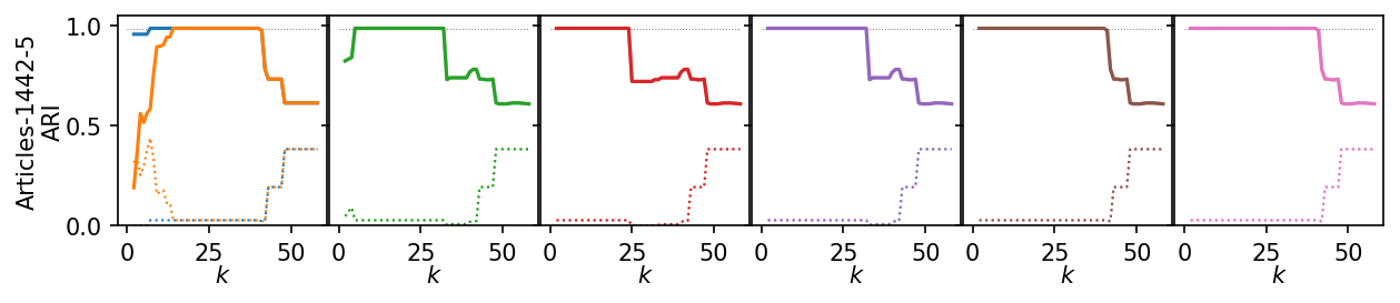
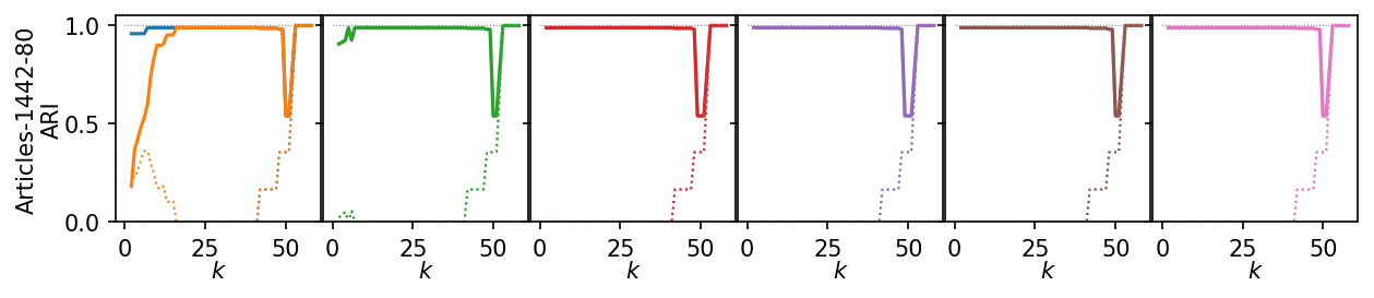
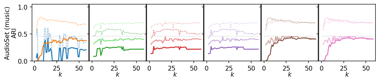
Now, we plot the ARI as a curve over \(k\). We interested in the range of \(k\) values for which the algorithms produce high quality clusterings.
[17]:
# Create the plots
plt.figure(figsize=(2.75 * 3, 0.6))
max_x = plot_df.k.max()
ticks = [0, 0.5, 1]
alg_idxs = [[0, 1], [2, 3], [4, 5], [6, 7], [8, 9], [10, 11]]
for j, ids in enumerate(alg_idxs):
    plt.subplot(1, 6, j + 1)
    plt.title(titles[j], y=0)
    plt.xlim(0, max_x)
    plt.xticks([0, 25, 50])
    plt.yticks([])
    plt.ylim(0, 1)
    if j == 0:
        plt.ylabel(f"{dataset_name(data_sets[0])}\nARI.", labelpad=0, color="w")
    plt.tick_params(axis="x", colors="white")
    plt.tick_params(axis="y", colors="white")
    plt.suptitle("Per dataset curves", y=1)
    plt.subplots_adjust(bottom=0, right=1, top=1, left=0.08, wspace=0.01)
    frame_off()

[18]:
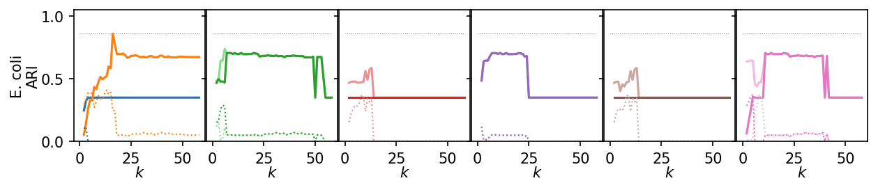
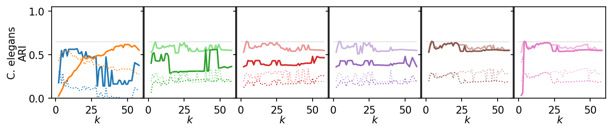
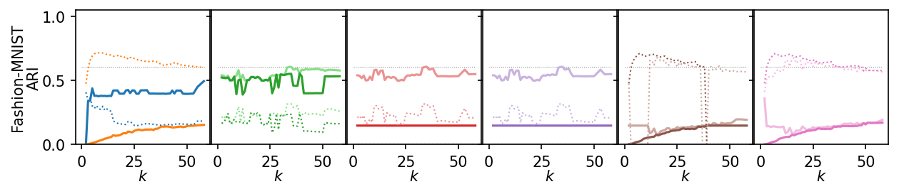
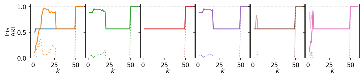
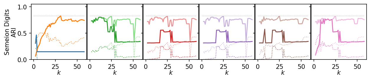
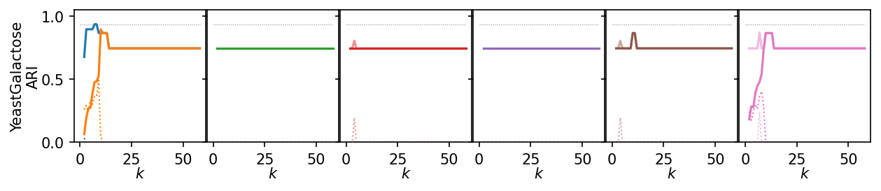
for i, data_name in enumerate(data_sets):
    plt.figure(figsize=(2.75 * 3, 1.75))
    ddf = plot_df.query(f'data_set == "{data_name}"')
    max_x = ddf.k.max()
    max_y = ddf.ari.max()
    for j, ids in enumerate(alg_idxs):
        plt.subplot(1, 6, j + 1)
        # frame_off()
        plt.hlines(
            max_y,
            0,
            max_x,
            colors=lighten("k"),
            linestyles=":",
            linewidth=0.5,
        )
        sns.lineplot(
            data=ddf,
            x="k",
            y="ari",
            hue="alg_id",
            hue_order=[alg_ids[idx] for idx in ids],
            errorbar=None,
            palette=[palette[idx] for idx in ids],
            legend=False,
        )
        sns.lineplot(
            data=ddf,
            x="k",
            y="noise_fraction",
            hue="alg_id",
            hue_order=[alg_ids[idx] for idx in ids],
            errorbar=None,
            palette=[palette[idx] for idx in ids],
            linestyle=":",
            linewidth=1,
            legend=False,
        )
        plt.xlabel("$k$", labelpad=0)
        plt.xticks([0, 25, 50])
        plt.ylim(0, 1.05)
        plt.yticks(ticks)
        if j == 0:
            plt.ylabel(f"{dataset_name(data_name)}\nARI", labelpad=0)
        else:
            plt.ylabel("")
            plt.gca().set_yticklabels(["" for t in ticks])
        plt.subplots_adjust(bottom=0.26, right=1, left=0.08, wspace=0.01, top=0.98)
plt.show()
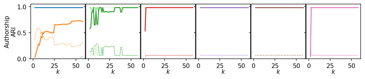
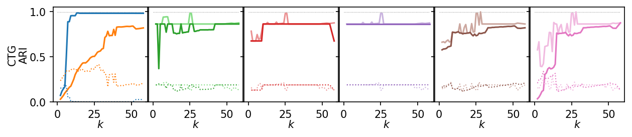
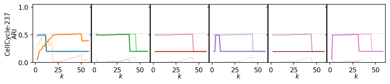
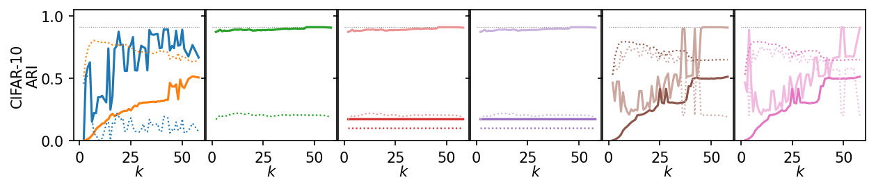
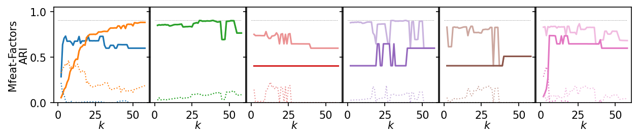
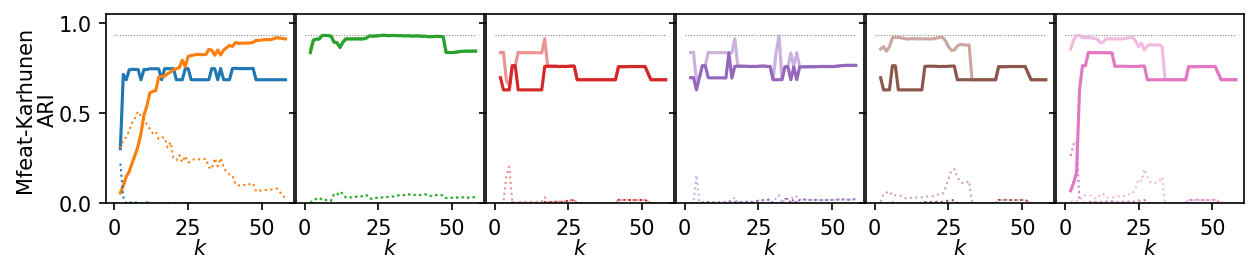
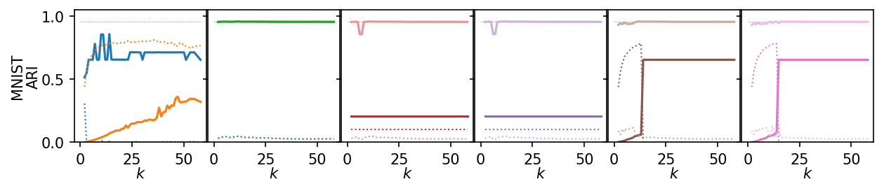
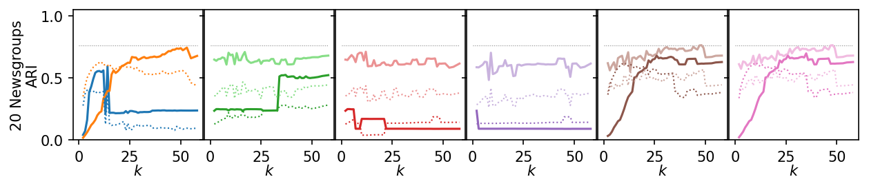
Next, we summarize the shape of the curves over all datasets by Lowess interpolation. We scaled the ARI scores by the maximum value achieved on each dataset to compare the curves, rather than the exact values. Still, this interpolation has issues because some datasets need other \(k\) values to get good clusters.
[19]:
def scale_quality(group):
    max_q = group.ari.max()
    group["scaled_quality"] = group.ari / max_q
    return group


plot_df = (
    plot_df.groupby(["data_set"])
    .apply(scale_quality, include_groups=False)
    .reset_index()
)
[20]:
plt.figure(figsize=(2.75 * 3, 2))
max_y = plot_df.scaled_quality.max()
for j, ids in enumerate(alg_idxs):
    plt.subplot(1, 6, j + 1)
    for i, idx in enumerate(ids):
        alg_id = alg_ids[idx]
        plt.hlines(max_y, 0, max_x, colors="k", linestyles=":", linewidth=0.5)
        regplot_lowess_ci(
            plot_df.query(f'alg_id == "{alg_id}"'),
            x="k",
            y="scaled_quality",
            ci_level=95,
            n_boot=100,
            lowess_frac=0.05,
            color=palette[idx],
            scatter=False,
        )
        plt.title(titles[j])
        plt.xlabel("k", labelpad=0)
        plt.ylim(0, 1)
        plt.yticks([])
        plt.xticks([0, 25, 50])
        if j == 0:
            plt.ylabel("Scaled ARI", labelpad=0)
        else:
            plt.ylabel("")
plt.suptitle("Interpolated ARI curves", y=1)
plt.subplots_adjust(bottom=0.22, right=1, left=0.02, wspace=0.02, top=0.68)
plt.show()
100%|██████████| 6307/6307 [38:33<00:00, 261.05it/s]

3. Compute sensitivity
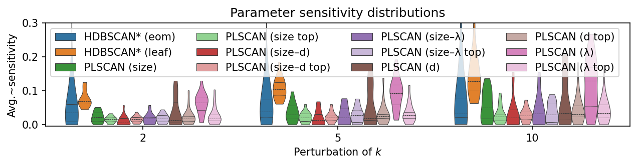
Now, we actually compute and compare the sensitivity measure. The measure describes how much quality scores change when the \(k\) parameter changes. So, it already takes into account absolute quality differences between datasets.
[21]:
sensitivity_records = []
for data_set, alg_id in product(df_top.data_set.unique(), df_top.alg_id.unique()):
    sub_df = df_top.query(f"data_set == '{data_set}' & alg_id == '{alg_id}'")
    vals = defaultdict(lambda: np.nan, {k: v for k, v in zip(sub_df.k, sub_df.ari)})
    lookup_fun = np.vectorize(lambda x: vals[x])
    initial_val = lookup_fun(min_sample_sizes)[np.newaxis, :, :]
    perturbed_val = lookup_fun(new_values)
    with np.errstate(divide="ignore", invalid="ignore"):
        diff = np.abs((perturbed_val - initial_val) / (perturbed_val + initial_val))
    with warnings.catch_warnings():
        warnings.simplefilter("ignore", category=RuntimeWarning)
        sensitivity = np.nanmean(diff, axis=(1, 2))
    for delta, sensitivity in zip(deltas[:, 0], sensitivity):
        sensitivity_records.append(
            {
                "data_set": data_set,
                "alg_id": alg_id,
                "perturbation": delta,
                "sensitivity": sensitivity,
            }
        )

# Convert to pandas
df_sens = pd.DataFrame.from_records(sensitivity_records)
df_sens.head()
[21]:
| data_set | alg_id | perturbation | sensitivity | |
|---|---|---|---|---|
| 0 | iris | plscan_size | 2 | 0.013380 |
| 1 | iris | plscan_size | 5 | 0.034243 |
| 2 | iris | plscan_size | 10 | 0.093711 |
| 3 | iris | plscan_distance | 2 | 0.005508 |
| 4 | iris | plscan_distance | 5 | 0.018361 |
On these datasets, PLSCAN has a lower sensitivity to \(k\) than HDBSCAN*. However, Peng et al. classify all values below 0.25 as insensitive.
[22]:
plt.figure(figsize=(2.8 * 3, 2))

plot_df = df_sens.copy()
plot_df.alg_id = plot_df.alg_id.apply(to_display_name)

alg_order = [0, 1, 3, 2, 5, 4, 7, 6, 9, 8, 11, 10]
hue_order = [to_display_name(alg_ids[x]) for x in alg_order]
alg_palette = [palette[x] for x in alg_order]
ax = sns.violinplot(
    data=plot_df,
    y=plot_df.sensitivity,
    x=pd.Categorical(plot_df.perturbation),
    hue=plot_df.alg_id,
    hue_order=hue_order,
    density_norm="count",
    palette=alg_palette,
    legend=True,
    inner="quartiles",
    linewidth=0.5,
    cut=0,
)
max_y = 0.3
plt.ylim(-0.005, max_y)
plt.legend(ncol=4, title="", loc="upper left")
plt.xlabel("Perturbation of $k$")
plt.ylabel("Avg.~sensitivity")
plt.title("Parameter sensitivity distributions")
plt.subplots_adjust(left=0.075, right=1, bottom=0.21, top=0.9)
plt.show()
4. Explore specific datasets
[23]:
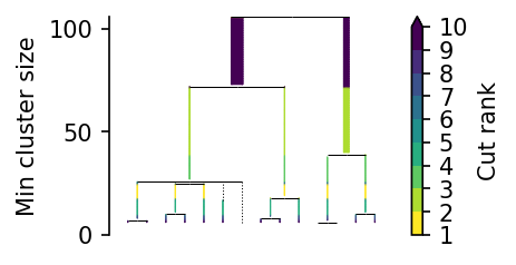
X = np.load("data/generated/benchmark_sensitivity_yeast_galactose_embedding.npy")
c = PLSCAN().fit(X)
c.leaf_tree_.plot()
plt.show()
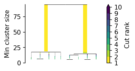
[24]:
df.data_set.unique()
[24]:
<ArrowStringArray>
[            'iris',            'mnist',    'fashion_mnist',
  'articles_1442_5', 'articles_1442_80',         'audioset',
       'authorship', 'cardiotocography',   'cell_cycle_237',
         'cifar_10',            'ecoli',          'elegans',
    'mfeat_factors',   'mfeat_karhunen',       'newsgroups',
          'semeion',  'yeast_galactose']
Length: 17, dtype: str
[25]:
y = np.load("data/ecoli/generated/y.npy")
u, c = np.unique(y, return_counts=True)
c
[25]:
array([143, 77, 2, 2, 35, 20, 5, 52])
[26]:
X = np.load("data/generated/benchmark_sensitivity_ecoli_embedding.npy")
c = PLSCAN().fit(X)
c.leaf_tree_.plot()
plt.show()