Cluster selection strategies

This notebook explains the HDBSCAN and PLSCAN cluster selection strategies and shows the effects of the min_samples and min_cluster_size parameters.

import warnings
import numpy as np
from hdbscan import HDBSCAN
from fast_plscan import PLSCAN
from lib.plotting import plt, fontsize, frame_off

plt.rcParams["figure.dpi"] = 150
plt.rcParams["figure.figsize"] = (2.75, 0.618 * 2.75)
data = np.load("data/clusterable/sources/clusterable_data.npy")

The function below runs the algorithms and plots their output in a nice overview.

def plot_parameter_sweep(title, alg, leaf_width="distance", **kwargs):
    """Plots the clusters and cluster hierarchies detected by the given
    algorithm at several min_samples / min_cluster_size values."""
    plt.figure(figsize=(2.75 * 3, 2.75))
    for i, size in enumerate([2, 5, 10, 50, 100]):
        with warnings.catch_warnings():
            warnings.simplefilter("ignore", FutureWarning)
            c = alg(min_samples=size, min_cluster_size=size, **kwargs).fit(data)
        plt.subplot(2, 5, i + 1)
        plot_kwargs = dict(s=1, cmap="tab10", vmax=9, vmin=0, edgecolors="none")
        plt.scatter(*data.T, c=c.labels_ % 10, **plot_kwargs)
        plt.title(f"$k={size}$", y=0.9)
        frame_off()

        plt.subplot(2, 5, i + 6)
        if alg == HDBSCAN:
            palette = plt.cm.tab10.colors
            c.condensed_tree_.plot(
                select_clusters=True,
                colorbar=False,
                leaf_separation=0.5,
                selection_palette=palette,
            )

        else:
            c.leaf_tree_.plot(
                select_clusters=True,
                colorbar=False,
                leaf_separation=0.5,
                width=leaf_width,
            )
        plt.ylabel("")
        plt.yticks([])
    plt.subplot(2, 5, 6)
    if alg == PLSCAN:
        plt.ylabel("Min. size", labelpad=0)
    else:
        plt.ylabel(r"$\lambda$ value", labelpad=0)
    plt.suptitle(title, y=1, fontsize=fontsize["normal"])
    plt.subplots_adjust(left=0.03, top=0.9, right=1, bottom=0, hspace=0, wspace=0.05)

HDBSCAN* cluster selection

HDBSCAN simplifies single linkage dendrograms using a minimum cluster size to create a cluster hierarchy (condensed_tree). The cluster hierarchy forms a merge-tree listing which connected components exist over all density values. As density decreases, larger distance edges enter the filtration and create connections between connected components, merging them in the hierarchy. The process describes the data’s 0-dimensional topology in a filtration over the density, effectively implementing a persistent homology computation.

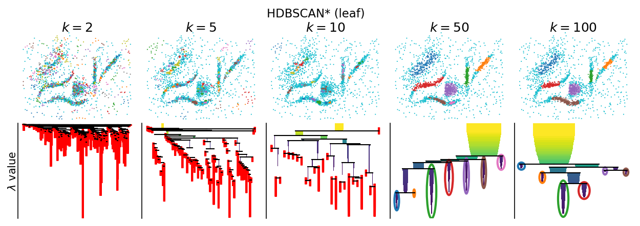
Clusters are selected from the hierarchy using one of two selection strategies. The leaf strategy always selects the cluster tree’s leaves. These clusters correspond to all local density maxima meeting the size threshold. Effectively, this strategy defines clusters as local density maxima. In practice, leaf-clusters depend strongly on the minimum cluster size value used to construct the cluster hierarchy. Many small leaf clusters can be detected for small minimum cluster sizes, resulting in segmentations where most points are classified as noise.

plot_parameter_sweep("HDBSCAN* (leaf)", HDBSCAN, cluster_selection_method="leaf")
plt.show()

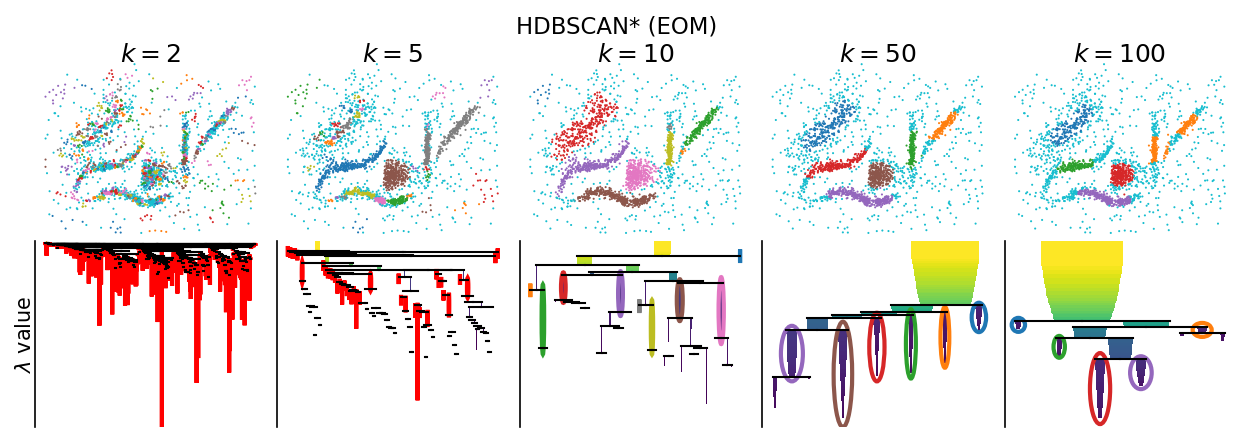
The EOM strategy is more statistically motivated. It encourages fewer, larger clusters by defining clusters as a neighborhoods with an excess of probability mass (explained by Müller & Sawitzki, 1991). In statistical terms, the EOM strategy interprets the density profile as a probability distribution and computes its modality. Specifically, the strategy selects connected components from the hierarchy that maximize a (relative) stability measure. The stability measure aggregates the density-ranges in which points are part of a particular connected component. It combines the number of points contained in the component with the points’ persistence in the density filtration. Selecting the most persistent structures from a filtration as the true signal is common in persistent homology and clustering (see, cluster lifetime referenced by Campello et al., 2015). The stability adapts this notion to a cluster with changing membership over density (Campello et al., 2015). While EOM clusters are less sensitive to the minimum cluster size, they vary enough that the parameter needs to be tuned to avoid small low-density clusters. Notice that some clusters disappear at larger size thresholds.

plot_parameter_sweep("HDBSCAN* (EOM)", HDBSCAN, cluster_selection_method="eom")
plt.show()

Both selection strategies can select clusters with varying densities that do not correspond to a straight density-cut in the cluster hierarchy. In other words, there may not be a single distance or density value for which DBSCAN produces the same clusters.

Persistent leaf-clusters

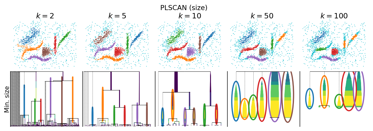
PLSCAN selects clusters by finding a minimum cluster size for which leaf-clusters are optimal. Like EOM, the resulting clusters relate to the density distributions modality, rather than all local maxima.

The strategy performs a very efficient filtration over the minimum cluster size parameter to create a leaf-cluster tree over all possible minimum cluster sizes. It then finds the min_cluster_size parameter that maximizes a quality measure. The result is a (practically) parameter free clustering algorithm that produces EOM-like clusters and a cluster hierarchy describing leaf-clusters at other size thresholds.

The min_samples parameter in PLSCAN smooths the computed density profile which prunes small, low-persistent leaves from the the leaf-cluster tree. Unlike hdbscan’s minimum cluster size parameter, changing ``min_samples`` in PLSCAN does not really change which clusters are selected. At higher min_samples the selected clusters becomes smaller, with more points classified as noise. This suggests low min_samples values work better. However, at too low values (i.e., min_samples=2 below), the resulting clusters might to sensitive to local density changes.

plot_parameter_sweep("PLSCAN (size)", PLSCAN)
plt.show()

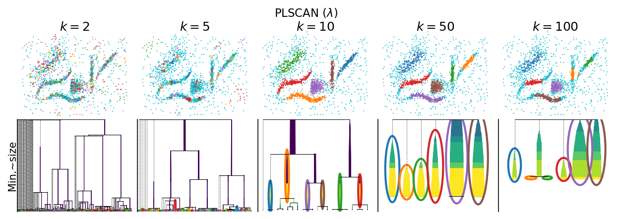
The other size-based persistence measures behave similarly:

• distance persistence

plot_parameter_sweep("PLSCAN ($d$)", PLSCAN, persistence_measure="distance")
plt.show()

• density persistence

plot_parameter_sweep("PLSCAN ($\\lambda$)", PLSCAN, persistence_measure="density")
plt.show()

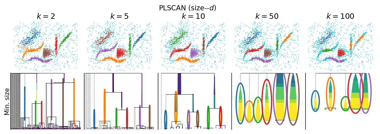
• size–distance bi-persistence

plot_parameter_sweep("PLSCAN (size--$d$)", PLSCAN, persistence_measure="size-distance")
plt.show()

• size–density bi-persistence

plot_parameter_sweep(
    "PLSCAN (size--$\\lambda$)",
    PLSCAN,
    persistence_measure="size-density",
    leaf_width="density",
)
plt.show()