Exploration plots

PLSCAN exposes several attributes for inspecting and visualizing its cluster hierarchy.

import numpy as np
import matplotlib.pyplot as plt
from fast_plscan import PLSCAN

plt.rcParams["figure.dpi"] = 150
plt.rcParams["figure.figsize"] = (2.75, 0.618 * 2.75)

data = np.load("data/clusterable/sources/clusterable_data.npy")

Condensed tree

Like HDBSCAN*, PLSCAN provides a condensed tree that summarizes how clusters merge as mutual reachability distance increases. Each branch represents a cluster lineage, and branch joins indicate merge events.

In PLSCAN visualizations, the tree is shown using distance-based quantities, which makes distance cuts directly interpretable.

c = PLSCAN().fit(data)

c.condensed_tree_.plot(select_clusters=True)
plt.show()

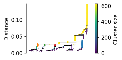
The distance_cut() method can be used to extract clusters at a given distance:

labels, probs = c.distance_cut(0.015)
plt.scatter(*data.T, c=labels % 10, s=1, alpha=0.4, linewidth=0, cmap="tab10")
plt.axis("off")
plt.show()

Leaf tree

PLSCAN does not select final clusters directly from the condensed tree. Instead, it builds a leaf-tree hierarchy that tracks which clusters are leaves (clusters with no child clusters) at each minimum cluster size threshold. The leaf_tree_ attribute stores this hierarchy:

c = PLSCAN().fit(data)

c.leaf_tree_.plot(select_clusters=True, leaf_separation=0.1)
plt.show()

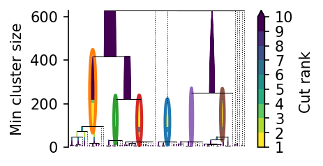
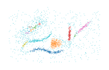
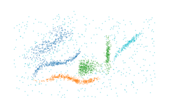
The min_cluster_size_cut() method can be used to extract clusters at a given minimum cluster size:

labels, probs = c.min_cluster_size_cut(300)
plt.scatter(*data.T, c=labels % 10, s=1, alpha=0.4, linewidth=0, cmap="tab10")
plt.axis("off")
plt.show()

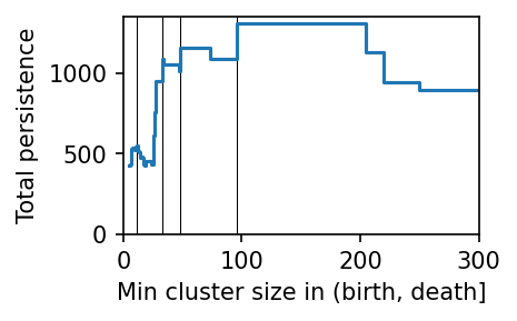
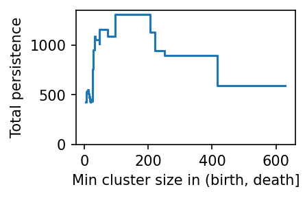
Persistence trace

PLSCAN selects clusters from the leaf tree by computing each leaf cluster’s persistence and finding the minimum cluster size threshold with the highest total persistence. The persistence_trace_ attribute visualizes this minimum-cluster-size vs persistence curve.

c.persistence_trace_.plot()
plt.show()

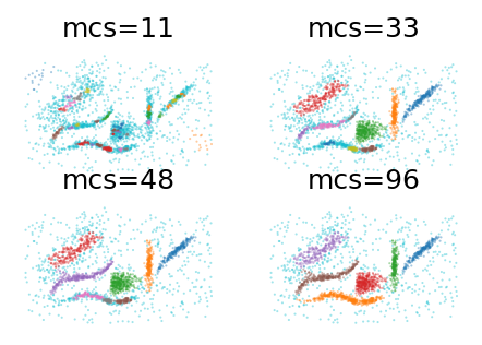
By default, PLSCAN selects the minimum cluster size threshold with the highest persistence value. Other robust alternatives can be explored with the cluster_layers method:

layers = c.cluster_layers(max_peaks=4)

for i, (size, labels, probs) in enumerate(layers):
    plt.subplot(2, 2, i + 1)
    plt.scatter(*data.T, c=labels % 10, s=1, alpha=0.4, linewidth=0, cmap="tab10")
    plt.title(f"mcs={int(size)}")  # mcs = min cluster size
    plt.axis("off")
plt.subplots_adjust(left=0, right=1, top=1, bottom=0)
plt.show()

These interesting clusterings relate to peaks in the minimum_cluster_size–persistence curve:

c.persistence_trace_.plot()
plt.vlines(list(zip(*layers))[0], *plt.ylim(), color="k", linewidth=0.5, zorder=1)
plt.xlim([0, 300])
plt.show()