Centroids, Medoids, and Exemplars

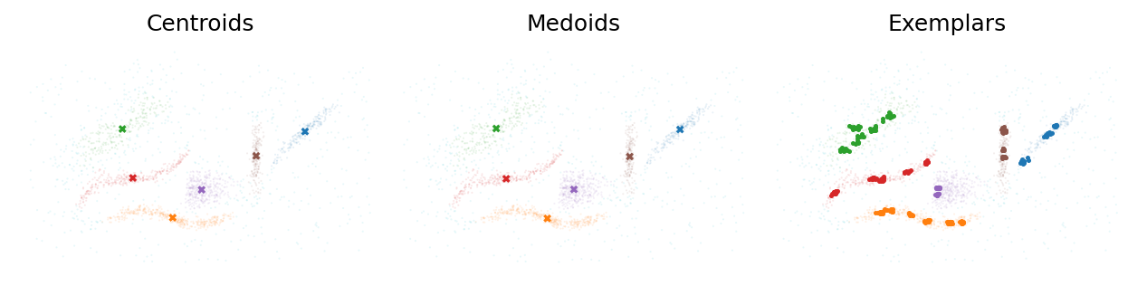
PLSCAN can efficiently compute cluster centers either as average feature coordinates (centroid), most central data points (medoid), or by finding the most dense data points (exemplars).

First, lets load the data again.

import numpy as np
import matplotlib.pyplot as plt


plt.rcParams["figure.dpi"] = 150
plt.rcParams["figure.figsize"] = (2.75, 0.618 * 2.75)

data = np.load("data/clusterable/sources/clusterable_data.npy")

The sklearn estimator PLSCAN has member-functions to compute centroids, medoids and exemplars.

from fast_plscan import PLSCAN

c = PLSCAN(min_samples=10).fit(data)
centroids = c.compute_centroids()
medoids = data[c.compute_medoid_indices(), :]
exemplars = [data[indices, :] for indices in c.compute_exemplar_indices()]

Centroids and medoids tend to be similar on Euclidean distances. For other distance methods, medoids are more appropriate. Exemplars provide more detail

about a cluster’s shape. As a result, they are used to cross-cluster membership

probabilities in the fast_plscan.prediction module.

plt.figure(figsize=(3 * 2.75, 0.618 * 2.75))
plt.subplot(1, 3, 1)
plt.scatter(*data.T, c=c.labels_ % 10, s=1, linewidth=0, cmap="tab10", alpha=0.1)
plt.scatter(
    *centroids.T, c=np.arange(len(centroids)), s=10, marker="x", cmap="tab10", vmax=9
)
plt.title("Centroids")
plt.axis("off")

plt.subplot(1, 3, 2)
plt.scatter(*data.T, c=c.labels_ % 10, s=1, linewidth=0, cmap="tab10", alpha=0.1)
plt.scatter(
    *medoids.T, c=np.arange(len(medoids)), s=10, marker="x", cmap="tab10", vmax=9
)
plt.title("Medoids")
plt.axis("off")

plt.subplot(1, 3, 3)
plt.scatter(*data.T, c=c.labels_ % 10, s=1, linewidth=0, cmap="tab10", alpha=0.1)
for i, explrs in enumerate(exemplars):
    plt.scatter(*explrs.T, color=f"C{i}", s=2)
plt.title("Exemplars")
plt.axis("off")

plt.subplots_adjust(0, 0, 1, 1, 0, 0)
plt.show()